
What is Minimum Variance Portfolio? Definition Meaning

minimum variance portfolio Breaking Down Finance

PPT Optimal risky portfolio PowerPoint Presentation ID

PPT La Frontera Eficiente de Inversión PowerPoint

FINDING MINIMUM VARIANCE PORTFOLIO FOR A 2ASSET

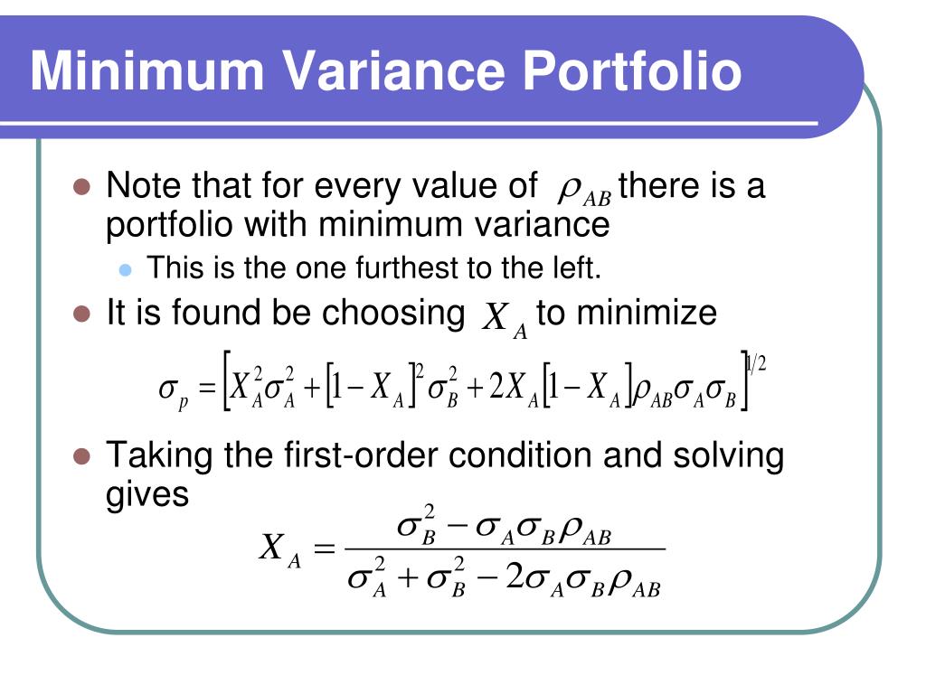
PPT Chapter 5 The Mathematics of Diversification

Note that covariance and correlation are mathematically related.
Minimum varianz portfolio formel. W ′ 1 = 1. This means that, instead of using both risk and return information as in the markowitz portfolio selection, the portfolio is constructed using only measures of risk. $\begingroup$ it's not a coding issue so much as it's the result of using long short portfolios.
S 1 = the standard deviation on. In particular, the video details how to graph an efficient frontier and f. The set of minimum variance portfolios is represented by a parabolic curve in the σ2 p − µp plane.
You are free to use this image on your website, templates etc, please provide us with an attribution link. This would tell us what proportions of the two assets to use (for any amount x 0 > 0 invested) to ensure the smallest risk. Northerntrust.com | minimum variance portfolio | 3 of 16 from equation 3 we have:
1 2 var ( w) = 1 2 w ′ σ w → min w s.t. Wte = 1 is called the feasible set, where each point corresponds to a portfolio with the constraints met. W1 and w2 are the percentage of each stock in the portfolio.
Andrew calculates the portfolio variance by adding the individual values of each stocks: Hence, the global minimum variance portfolio has portfolio weights = 0 4411 =0 3656 and =0 1933 and is given by the vector m =(0 4411 0 3656 0 1933)0 (1.9) the expected return on this portfolio, = m0μ is > mu.gmin = as.numeric(crossprod(m.vec, mu.vec)) > mu.gmin It is the solution of the problem.
The same formula applies for each weight, thus deriving the total optimized returns for each stock, as follows: Portfolio variance = 0.0006 + 0.0007 + 0.0006 + 0.0016 + 0.0005 = 0.0040 = 0.40%. Mathematically, the portfolio variance formula consisting of two assets is represented as, portfolio variance formula = w12 * ơ12 + w22 * ơ22 + 2 * ρ1,2 * w1 * w2 * ơ1 * ơ2.

Global Minimum Variance 2 System of Equations YouTube

Minimum Variance Portfolio ver 1 YouTube

Solactive Diversification The Power of Bonds

Minimum Variance Portfolios Mathematics and Derivation

Lecture 51 What is Portfolio Variance? YouTube

PPT FINC4101 Investment Analysis PowerPoint Presentation

Capm
PPT Investment Analysis and Portfolio Management

1635 variance portfolio

5 MINIMUM VARIANCE PORTFOLIO HOW TO CALCULATE, MINIMUM

Portfolio Theory Calculating a Minimum Variance Two Asset

Portfolio Theory Calculating a Minimum Variance Two Asset

5 MINIMUM VARIANCE PORTFOLIO HOW TO CALCULATE, MINIMUM

