
How To Download Pie Charts From Google Forms Chart Walls

How to Make a Pie Chart in Google Sheets How To NOW

How to create Pie Chart or Graph in Google Sheets YouTube

How to Make a Graph or Chart in Google Sheets

How to Make Professional Charts in Google Sheets Pie chart template

Google sheets chart tutorial how to create charts in google sheets
At the right, click customize.
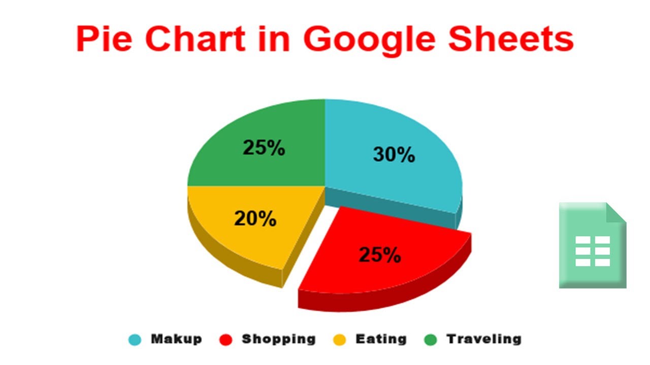
How to make a pie chart using google sheets. Add a slice label, doughnut hole, or change border. Choose the data you want to make a pie chart (including header). To customize the pie chart, click anywhere on the chart.
Select the range of data that you want to visualize. Then click the three vertical dots in the top right corner of the chart. To edit a chart you’ve already created, first open the chart editor for that graph by selecting the chart and clicking on the 3 dot menu icon in the corner of the chart.
Click on the chart icon from the toolbar. Then click move to own sheet. A chart editor will open on the right.
An array of objects, each describing the format of the corresponding slice in the pie. Click on the “pie chart” dropdown to open up the pie chart options. November 21, 2018 at 6:21 am.
Select “chart style” from the available options to bring up the chart editor panel. Download this free how to make a pie chart in google sheets article in pdf. Usually, the default chart isn’t a pie chart but don’t worry as we’ll change that in a.
Here are the steps in creating a pie chart from an existing dataset in google sheets: In the dropdown that appears after. This covers the basics of creating a pie chart, but the instructions apply to bar charts, line charts, etc.

How to change the values of a pie chart to absolute values instead of

How to Make a Pie Chart in Google Sheets from a PC, iPhone or Android

Creating a Pie Chart in Google Sheets YouTube

